Oh control. Who doesn't enjoy having control of things in life every so often? While many of us probably wish life could be more easily controlled, alas things often have too much chaos to be adequately predicted and in turn controlled. While lack of complete controllability is the case for many things in life, like getting the ultimate job or getting even one for that matter (sorry I'm a Millenial), there are still plenty of things that can be controlled.. And many are controlled by engineers.

While controlling systems is a challenge, especially if they are nonlinear, stochastic, partially controllable, etc., there is a wealth of work that has been done to tackle these problems. Now, it is useful to gain familiarity with some of these mathematical tools successfully used in control problems. One interesting tool is that of Optimal Control.

In this blog post, I'm going to cover the use of Dynamic Programming to tackle deterministic Discrete-Time Linear Control problems for the case of bringing the state to $\boldsymbol{0}$. I will also assume for simplicity all states are observable. With this tool, one will have a useful formulation that can be used to approximately tackle control problems in some optimal sense.

The Formulation

The Dynamics

In the general deterministic, nonlinear dynamics formulation, we can represent the dynamics in a State Space form written as shown below:

\begin{align} \frac{d \boldsymbol{x}}{dt} &= f(t,\boldsymbol{x},\boldsymbol{u}) \end{align}

where $t \in \mathbb{R}$ is the time, $\boldsymbol{x} \in \mathbb{R}^n$ is the state vector, $\boldsymbol{u} \in \mathbb{R}^m$ is the control vector, and $f(\cdot,\cdot)$ is mapping used to compute the time derivative of the state vector, defined as the following:

\begin{align} f &: \mathbb{R} \times \mathbb{R}^n \times \mathbb{R}^m \rightarrow \mathbb{R}^n \end{align}

Given we have the dynamics written in this differential form, we can convert it to a discrete form by approximating the time derivative of $\boldsymbol{x}$ with a simple Finite Difference formula. Thus, we can derive the discrete form in the following way:

\begin{align} \left.\frac{d \boldsymbol{x}}{dt}\right|_{t_k} &= f(t_k,\boldsymbol{x}_k,\boldsymbol{u}_k) \nonumber \\ \frac{\boldsymbol{x}_{k+1} - \boldsymbol{x}_k }{\Delta t} &\approx f(t_k,\boldsymbol{x}_k,\boldsymbol{u}_k) \nonumber \\ \boldsymbol{x}_{k+1} &\approx \boldsymbol{x}_k + \Delta t f(t_k,\boldsymbol{x}_k,\boldsymbol{u}_k) \end{align}

Now we can assume the system is linear, making the actual discrete-time system of the following form:

\begin{align} \boldsymbol{x}_{k+1} &\approx A_{k}\boldsymbol{x}_k + B_{k}\boldsymbol{u}_k \end{align}

where $A_{k}$ and $B_{k}$ are matrices that can be dependent on time. With this discrete form, we have one of the main ingredients needed to approach optimal control problems using Dynamic Programming. Next, we need to investigate how we will define optimality.

The Cost Function

For many optimal control problems, we can get away with using a cost function of the form shown below:

\begin{align} J &= \left.\left( \boldsymbol{x}^{T}(t) Q_f \boldsymbol{x}(t)\right)\right|_{t=t_N} + \sum_{k=1}^{N-1} \left.\left( \boldsymbol{x}^{T}(t) Q(t) \boldsymbol{x}(t) + \boldsymbol{u}^{T}(t) R(t) \boldsymbol{u}(t) \right)\right|_{t=t_k} \nonumber \\ &= \boldsymbol{x}^{T}_N Q_f \boldsymbol{x}_N + \sum_{k=1}^{N-1} \left( \boldsymbol{x}^{T}_k Q_k \boldsymbol{x}_k + \boldsymbol{u}^{T}_k R_k \boldsymbol{u}_k \right) \\ \end{align}

The cost function shown above ends up being quadratic with respect to both the state and control vectors at each time that one cares to make the controller based on. Note that the matrices $Q_f$, $Q_k \forall k$, and $R_k \forall k$ are chosen by the control engineer to ensure desireable properties. The need to choose these various matrices for the cost function is one of the big parts that makes control engineer an art more than a science and benefits from lots of experience. Anyway, now that we have the cost function, we can start investigating how to obtain an optimal controller using Dynamic Programming!

The Dynamic Programming Approach

So when tackling some optimal control problem, you are essentially striving to find an optimal time history of both the state, $\boldsymbol{x}$, and the control, $\boldsymbol{u}$. This time history of values can be viewed as optimal paths for $\boldsymbol{x}$ and $\boldsymbol{u}$. Now the premise of Dynamic Programming is essentially that a single optimal path can be broken up into optimal sub-paths that are optimal in their own domain, yet when unioned together become the desired complete optimal trajectory.

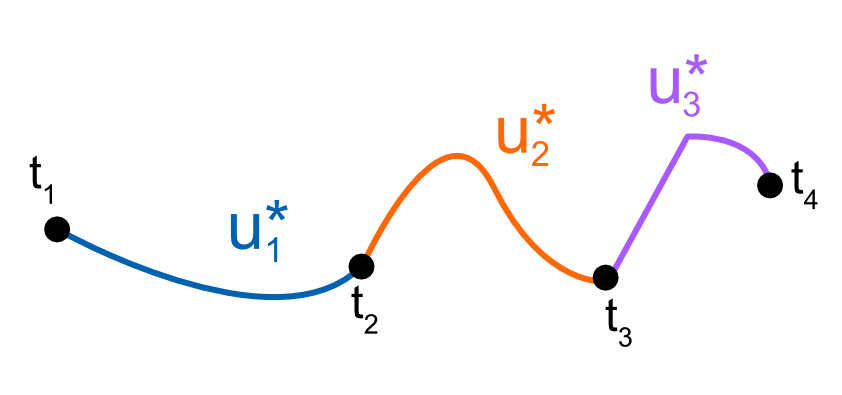
Using the concept behind Dynamic Programming, one should be able to obtain state and control trajectory in pieces and wind up with the overall optimal trajectories when you're done. So given that, where can we even begin to start coming up with an optimal trajectory?

Since we earlier wrote out the cost function we're going to use, we know that we have some desired end state and then a penalty cost based on the actual trajectory we take. Since we really want to end up with the final state, a smart strategy is to start at the end of the trajectory and work backwards in time! Might make sense, but that kind of sounds hard or even impossible.. Well to help us think this through, let's start out with a simpler control problem to illustrate the approach!

Scalar Dynamic Programming Control Problem

Working out some math

For this problem, let's assume the below scalar dynamics and cost function:

\begin{align} x_{k+1} &= \alpha x_{k} + \beta u_{k}\\ J &= Q_f x_{3}^2 + \sum_{k=1}^{2} Q x_{k}^2 + R u_{k}^2 \end{align}

Notice that the discrete dynamics for $x_{k+1}$ is linear with respect to $x_{k}$ and $u_{k}$. This is a simplification for the sake of the example, but real world problems will not necessarily be linear. We will investigate nonlinear problems in future posts, but for this post linear is what we will stick to! Now back to the problem... Since we want to work from the end back to the beginning, let's first assume our final cost is:

\begin{align} V_{3} &= Q_f x_{3}^2 \end{align}

We then know recursively the following costs exist for the other parts of the control problem:

\begin{align} V_{2} &= Q x_{2}^2 + R u_{2}^2 + V_{3}\\ V_{1} &= Q x_{1}^2 + R u_{1}^2 + V_{2} \end{align}

Notice how we have broken up our problem into successive pieces of the overall cost function. This strategy gives us an ability to recursively tackle finding optimal state and control trajectories piece by piece.

So let us first start with finding $u_{2}$, the last control action that will be taken in the sequence. Looking at $V_{2}$, we know that $V_{3}$ is dependent on $x_{3}$. Through our dynamics, we know we can relate $x_{3}$ to $u_{2}$ using the fact that $x_{3} = \alpha x_{2} + \beta u_{2}$. Substituting this into the $V_{2}$ equation in the $V_{3}$ term can work out to give use the following:

\begin{align*} V_{2} &= Q x_{2}^2 + R u_{2}^2 + V_{3}\\ &= Q x_{2}^2 + R u_{2}^2 + Q_f x_{3}^2\\ &= Q x_{2}^2 + R u_{2}^2 + Q_f \left(\alpha x_{2} + \beta u_{2}\right)^2\\ &= Q x_{2}^2 + R u_{2}^2 + Q_f\alpha^2 x_{2}^2 + Q_f \beta^2 u_{2}^2 + 2 Q_f \alpha \beta x_{2}u_{2}\\ &= \left(Q + Q_f \alpha^2 \right) x_{2}^2 + \left( R + Q_f \beta^2 \right) u_{2}^2 + 2 Q_f \alpha \beta x_{2}u_{2} \end{align*}

Now given our expression for $V_{2}$, let's compute the value for $u_{2}$ that minimizes it! Thus:

\begin{align} \frac{\partial V_{2}}{\partial u_{2}} = 0 &= 2 \left( R + Q_f \beta^2 \right) u_{2} + 2 Q_f \alpha \beta x_{2} \nonumber \\ u_{2} &= -\left( R + Q_f \beta^2 \right)^{-1} Q_f \alpha \beta x_{2}\\ &= -K_{2} x_{2} \end{align}

where we can see $u_{2}$ ends up as a feedback controller based on the state $x_{2}$ and $K_{2}$ is the linear control gain. That's pretty interesting! But so, how do we proceed to obtain $u_{1}$? Well, we first use our result for $u_{2}$ to get $V_{2}$ in terms of just $x_{2}$ and then apply the same process to $V_{1}$! Let's try it out:

\begin{align} V_{2} &= \left(Q + Q_f \alpha^2 \right) x_{2}^2 + \left( R + Q_f \beta^2 \right) u_{2}^2 + 2 Q_f \alpha \beta x_{2}u_{2} \nonumber \\ &= \left(Q + Q_f \alpha^2 \right) x_{2}^2 + \left( R + Q_f \beta^2 \right) K_{2}^2 x_{2}^2 - 2 K_{2} Q_f \alpha \beta x_{2}^2 \nonumber \\ &= \left(Q + Q_f \alpha^2 + (R + Q_f \beta^2)K_{2}^2 - 2 K_{2} Q_f \alpha \beta \right) x_{2}^2 \nonumber \\ &= P_{2} x_{2}^2 \end{align}

So now that we have worked out $V_{2}$ in terms of quantities we know and just with respect to $x_{2}$, we can apply the same steps from earlier to end up with the control $u_{1}$ by doing the following:

\begin{align*} V_{1} &= Q x_{1}^2 + R u_{1}^2 + V_{2}\\ &= Q x_{1}^2 + R u_{1}^2 + P_{2} x_{2}^2\\ &= Q x_{1}^2 + R u_{1}^2 + P_{2} \left(\alpha x_{1} + \beta u_{1}\right)^2\\ &= Q x_{1}^2 + R u_{1}^2 + P_{2} \alpha^2 x_{1}^2 + P_{2} \beta^2 u_{1}^2 + 2 P_{2} \alpha \beta x_{1}u_{1}\\ &= \left(Q + P_{2} \alpha^2 \right) x_{1}^2 + \left( R + P_{2} \beta^2 \right) u_{1}^2 + 2 P_{2} \alpha \beta x_{1}u_{1} \\ \frac{\partial V_{1}}{\partial u_{1}} = 0 &= 2 \left( R + P_{2} \beta^2 \right) u_{1} + 2 P_{2} \alpha \beta x_{1} \\ u_{1} &= -\left( R + P_{2} \beta^2 \right)^{-1} P_{2} \alpha \beta x_{1}\\ &= -K_{1} x_{1} \end{align*}

Very interesting! We have indeed found the feedback control formulas for the control actions needed to minimize the cost function we have defined. Now we did a simple problem, but have you been able to see a pattern in the algorithmic steps to finding the optimal control sequence? Using the following definitions, we can define a recursive equation to finding each gain needed to perform the optimal control action. Here are the following equations:

\begin{align} K_{k} &= (R + P_{k+1} \beta^2 )^{-1} P_{k+1} \alpha \beta \\ P_{k} &= Q + P_{k+1} \alpha^2 + (R + P_{k+1} \beta^2 )K_{k}^2 - 2 K_{k} P_{k+1} \alpha \beta \end{align}

where $k \in \lbrace 1, 2, \cdots, N-1 \rbrace$, $P_{N} = Q_f$, and we compute the feedback control via the equation:

\begin{align} u_{k} &= -K_{k} x_{k} \end{align}

To prove the worth of this equation, let us implement some codes and show the system is asymptotically stabilized, aka $x_{N}$ reaches a value near $0$.

Algorithmic Test of Control Formulation

Let's get this computational proof rolling by first implementing a function that will compute the sequential gains needed for the control problem. Below shows a Matlab code to do just that!

function [ K ] = getControlGains( alpha, beta, Qf, Q, R, N )
%GETCONTROLGAINS Method to get control gains sequence for linear scalar
% control problem tackled using Dynamic Programming
% Author: C. Howard
K = zeros(N-1,1);
P = Qf;
for i = (N-1):-1:1
 K(i) = (P*alpha*beta )/( R + P*beta);
 P = Q + P*alpha + (R+P*beta)*K(i)^2 - 2*K(i)*P*alpha*beta;
end
end

The next code is simply one that does a simple Monte Carlo sampling of tuning parameter values, simulates the control and dynamics based on them, and saves off a figure. This code can be found below:

% script to test control sequence
% for linear scalar control problem
% set constants
N = 500;    % number of control steps to use in algorithm
Qf = 2;    % final cost weighting
Q = 10;    % cost weighting of state
R = 80;    % cost weighting of control
dt = 1e-2;
alpha = (1-dt);
beta = dt.*1;
NMC = 10;
for i = 1:NMC
    
    Qf = rand()*20;   % final cost weighting
    Q  = rand()*10;   % cost weighting of state
    R  = rand()*150;  % cost weighting of control
    % Get Control Gains
    K = getControlGains(alpha,beta,Qf,Q,R,N);
    % Get ready to simulate
    x0 = 1;
    x = zeros(N,1);
    x(1) = x0;
    u = zeros(N-1,1);
    % Do simulation
    for i = 2:N
        u(i-1) = -K(i-1)*x(i-1);
        x(i) = alpha*x(i-1) + beta*u(i-1);
    end
    % plot results
    time = dt.*(0:N-1);
    figure(1)
    plot(time,x,'-','Color',[0.5,0,1.0],'LineWidth',2)
    hold on
    plot(time(1:end-1),u,'-','Color',[0.9,0,0.2],'LineWidth',2)
    grid on
    xlabel('Time','FontSize',16)
    ylabel('Value','FontSize',16)
    title({sprintf('$$Q_{f} = %0.2f | Q = %0.2f | R = %0.2f | \\alpha = %0.2f | \\beta = %0.2f$$',Qf,Q,R,alpha,beta)},'interpreter','latex','FontSize',16)
    legend({'x','u'},'Location','Best')
    hold off
    axis([0,time(end),-x0,x0])
    print(gcf,'-dpng','-r300',sprintf('plots/qf%0.2f_q%0.2f_r%0.2f_a%0.2f_b%0.2f_sim.png',Qf,Q,R,alpha,beta))
    close all;
end

Now below we see some results from the above code for different values of the tuning parameters:

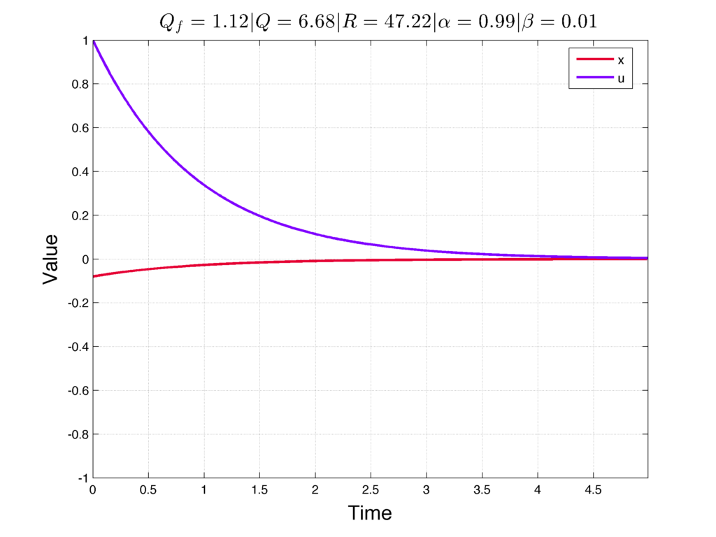
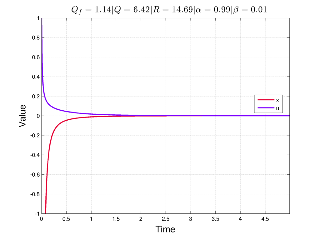
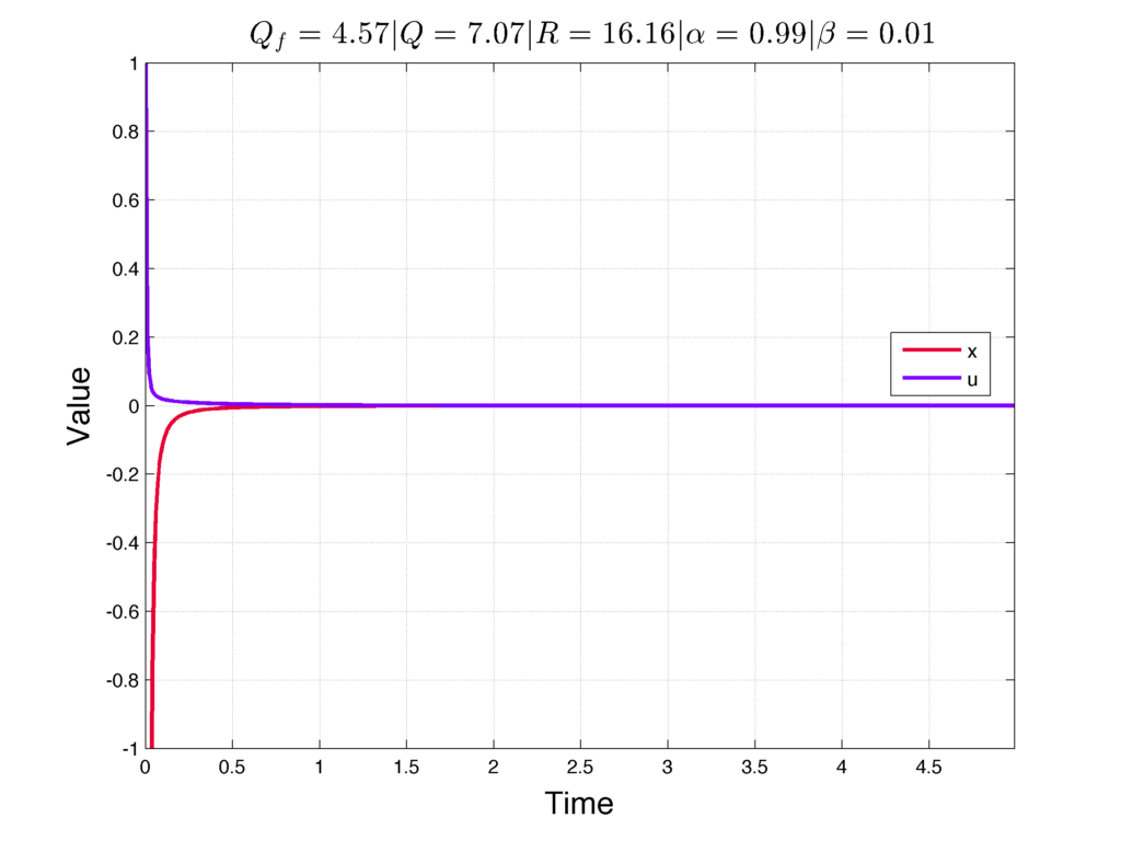
If one looks at these figures, we can see that smaller values for $R$ allows for $u$ to take on larger magnitudes at a given time. As $R$ increases, though, we see that the magnitude of $u$ reduces and in turn makes it take longer for the dynamical system to approach the desired steady state value of $0$.

This all makes sense since $R$ penalizes large magnitudes for $u$, meaning a large value for $R$ should shrink the magnitude of $u$ over the time history. Now if we were to set larger values for $Q_{f}$ and $Q$, we could expect the magnitude of $u$ to increase over the time history since the cost function would focus less on minimizing control and instead focus on getting the state to the desired steady state value. I think it is pretty neat seeing how the tuning variables can intuitively affect the control performance!

Now this was all for a scalar problem, but how about we extend this to Linear Multiple Input Multiple Output (MIMO) systems!

Linear MIMO Dynamic Programming Control Problem

Working out some math

Let us first assume the dynamics can be written like the following:

\begin{align*} \boldsymbol{x}_{k+1} &= A_{k} \boldsymbol{x}_{k} + B_{k} \boldsymbol{u}_{k} \end{align*}

where $A_{k}$ and $B_{k}$ can be time varying matrices. Let's then define the Dynamic Programming cost recursively as the following:

\begin{align} V_{k} &= \boldsymbol{x}_{k}^{T}Q_{k}\boldsymbol{x}_{k} + \boldsymbol{u}_{k}^{T}R_{k}\boldsymbol{u}_{k} + \boldsymbol{x}_{k+1}^{T}P_{k+1}\boldsymbol{x}_{k+1} \\ P_{N} &= Q_{f} \end{align}

We can then substitute the Linear MIMO dynamics to replace the $\boldsymbol{x}_{k+1}$ term in the recursive cost equation. This results in:

\begin{align} V_{k} &= \boldsymbol{x}_{k}^{T}Q_{k}\boldsymbol{x}_{k} + \boldsymbol{u}_{k}^{T}R_{k}\boldsymbol{u}_{k} + \left(A_{k} \boldsymbol{x}_{k} + B_{k} \boldsymbol{u}_{k}\right)^{T}P_{k+1}\left(A_{k} \boldsymbol{x}_{k} + B_{k} \boldsymbol{u}_{k}\right) \label{eq1} \end{align}

We can then take the derivative of $V_{k}$ with respect to $\boldsymbol{u}_{k}^{T}$ and solve for an optimal value for $\boldsymbol{u}_{k}$ by doing the following:

\begin{align*} \frac{\partial V_{k}}{\partial \boldsymbol{u}_{k}^{T}} = 0 &= 2 R_{k}\boldsymbol{u}_{k} + 2 B_{k}^{T}P_{k+1}\left(A_{k} \boldsymbol{x}_{k} + B_{k} \boldsymbol{u}_{k}\right) \\ 0 &= \left( R_{k} + B_{k}^{T}P_{k+1}B_{k} \right) \boldsymbol{u}_{k} + B_{k}^{T}P_{k+1}A_{k} \boldsymbol{x}_{k} \\ \boldsymbol{u}_{k} &= -\left( R_{k} + B_{k}^{T}P_{k+1}B_{k} \right)^{-1} B_{k}^{T}P_{k+1}A_{k} \boldsymbol{x}_{k} \\ \boldsymbol{u}_{k} &= -K_{k} \boldsymbol{x}_{k} \end{align*}

where $K_{k} = \left( R_{k} + B_{k}^{T}P_{k+1}B_{k} \right)^{-1} B_{k}^{T}P_{k+1}A_{k}$. Now with the solution to the optimal control specified as $\boldsymbol{u}_{k} = -K_{k} \boldsymbol{x}_{k}$, we can make a substitution with the result and get a recursive expression for $P_{k}$ in terms of known quantities. Thus:

\begin{align} V_{k} &= \boldsymbol{x}_{k}^{T}Q_{k}\boldsymbol{x}_{k} + \boldsymbol{u}_{k}^{T}R_{k}\boldsymbol{u}_{k} + \left(A_{k} \boldsymbol{x}_{k} + B_{k} \boldsymbol{u}_{k}\right)^{T}P_{k+1}\left(A_{k} \boldsymbol{x}_{k} + B_{k} \boldsymbol{u}_{k}\right) \\ V_{k} &= \boldsymbol{x}_{k}^{T}Q_{k}\boldsymbol{x}_{k} + \boldsymbol{x}_{k}^{T}K_{k}^{T}R_{k}K_{k} \boldsymbol{x}_{k} + \boldsymbol{x}_{k}^{T}\left(A_{k} - B_{k}K_{k}\right)^{T}P_{k+1}\left(A_{k} - B_{k}K_{k}\right)\boldsymbol{x}_{k} \\ V_{k} &= \boldsymbol{x}_{k}^{T}\left(Q_{k} + K_{k}^{T}R_{k}K_{k} + \left(A_{k} - B_{k}K_{k}\right)^{T}P_{k+1}\left(A_{k} - B_{k}K_{k}\right)\right)\boldsymbol{x}_{k} \\ V_{k} &= \boldsymbol{x}_{k}^{T}P_{k}\boldsymbol{x}_{k} \\ \therefore P_{k} &= Q_{k} + K_{k}^{T}R_{k}K_{k} + \left(A_{k} - B_{k}K_{k}\right)^{T}P_{k+1}\left(A_{k} - B_{k}K_{k}\right) \end{align}

With this, our full recursive equations with the base case are the following:

\begin{align} K_{k} &= \left( R_{k} + B_{k}^{T}P_{k+1}B_{k} \right)^{-1} B_{k}^{T}P_{k+1}A_{k} \\ P_{k} &= Q_{k} + K_{k}^{T}R_{k}K_{k} + \left(A_{k} - B_{k}K_{k}\right)^{T}P_{k+1}\left(A_{k} - B_{k}K_{k}\right) \\ \boldsymbol{u}_{k} &= -K_{k} \boldsymbol{x}_{k} \\ P_{N} &= Q_{f} \end{align}

where $k \in \lbrace 1, 2, \cdots, N-1 \rbrace$. With these equations, given a fully observable Linear MIMO system, one can work backwards from some time $t_{N}$ and figure out the sequence of gain matrices, $K_{k} \forall k$, that minimize the quadratic cost function! This is really cool because now we have a pretty general set of equations that can be used for many real control problems!

Conclusion

In this post we have gone over some fundamentals of developing optimal controllers using Dynamic Programming to tackle Linear control problems. In future posts, we will seek to consider nonlinear dynamical systems. Diving into this more complicated area is much more challenging and will require a new post devoted to introducing the topic.

With all that said, we have conquered a lot of stuff in this post and have good reason to feel good about ourselves! There is only one thing left to say...