Hey there reader! It has been quite a while since I wrote a blog post.. but I have had a ton of things on my mind I wanted to write about! I am stoked to be able to write about some of them now!

Since leaving my job in defense to go to graduate school — yes, I am obviously into being a poor student — I have been busy with classes and research and have been introduced to some pretty cool new ideas. One awesome algorithm I was introduced to was related to the estimation of the Range (also called Column Space) of some matrix operator using a randomized algorithm.

To be more rigorous, we can define a matrix operator as $M: \mathbb{R}^n \rightarrow \mathbb{R}^m$ for $m \leq n$, meaning it maps an $n$-dimensional vector into an $m$-dimensional vector. The goal of the algorithm that will be introduced is to essentially find an approximate basis for the range of some matrix $M$ that spans $M$'s column space. Additionally, we would like to ideally estimate this basis with minimal computation. Time to see where we can go with this!

Baseline Approach

So given some matrix $M \in \mathbb{R}^{m \times n}$, it actually is not very tough to find a basis for the range of $M$. The easiest way one could do this would be to do a QR decomposition, i.e. $M = QR$, where the columns of $Q$ would represent orthogonal vectors that span the range of $M$. The sad thing about using this approach directly is the computational complexity is $O(m^2 n)$. Can we do better? The answer: we can.

Randomized Approach

So let us assume we know the approximate rank, $k$, of the matrix $M$ where $k \leq m \leq n$. Let us then assume we can generate some random set of input samples $\Omega \in \mathbb{R}^{n \times k}$ where each column of $\Omega$ is a random vector. If we assume we can compute each element of $\Omega$ in constant complexity, a randomized algorithm can proceed in the following steps with each associated computational complexity:

\begin{align} &\text{Construct random matrix $\Omega \in \mathbb{R}^{n \times k}$ } &\rightarrow &O(nk) \tag{1}\\ &\text{Get measurements from $A$ by doing $Y = A\Omega$ } &\rightarrow &O(mnk) \tag{2}\\ &\text{Perform QR of $Y \ni Y = QR$ } &\rightarrow &O(mk^2) \tag{3}\\ &\text{Return range estimate, $Q$} &\rightarrow &O(mk) \tag{4} \end{align}

The described algorithm has a dominating complexity of $O(mnk)$, potentially a huge speed up if $k \ll m$ and at least an improvement over the baseline approach which has an $O(m^2 n)$ complexity. The whole idea of this method is to use random inputs from $\Omega$ to extract information from the range of $M$ and then use a QR decomposition to actually use that information to estimate the basis that spans $M$'s range. If one wants to find the most dominant $k$ basis vectors more reliably, you can also throw in a power iteration styled loop into the algorithm. This can modify the algorithm into the following:

\begin{align} &\text{Construct random matrix $\Omega \in \mathbb{R}^{n \times k}$ } &\rightarrow &O(nk) \tag{1}\\ &\text{Get measurements from $A$ by doing $Y = A\Omega$ } &\rightarrow &O(mnk) \tag{2}\\ &\text{For some small constant $N$ iterations, do: } \tag*{}\\ &\quad\text{Perform QR of $Y \ni Y = QR$ } &\rightarrow &O(mk^2)\tag{i}\\ &\quad\text{Compute $U = A^T Q$ } &\rightarrow &O(mnk)\tag{ii}\\ &\quad\text{Perform QR of $U \ni U = QR$ } &\rightarrow &O(mk^2)\tag{iii}\\ &\quad\text{Compute $Y = AQ$ } &\rightarrow &O(mnk)\tag{iv}\\ &\text{Perform QR of $Y \ni Y = QR$ } &\rightarrow &O(mk^2) \tag{3}\\ &\text{Return range estimate, $Q$} &\rightarrow &O(mk) \tag{4} \end{align}

Note that, again, the overall computational complexity ends up being $O(mnk)$ but in this case the basis found that spans the range of $M$ will be much more precise thanks to the power iteration. For those that like to have some code to look at, the following function can be used to perform the above computation.

import numpy as np
def randproj(A, k, random_seed = 17, num_power_method = 5):
    # Author: Christian Howard
    # This function is designed to take some input matrix A
    # and approximate it by the low-rank form A = Q*(Q^T*A) = Q*B.
    # This form is achieved using randomized algorithms.
    # 
    # Inputs:
    # A: Matrix to be approximated by low-rank form
    # k: The target rank the algorithm will strive for.
    # random_seed: The random seed used in code so things are repeatable.
    # num_power_method: Number of power method iterations
    # set the random seed
    np.random.seed(seed=random_seed)

    # get dimensions of A
    (r, c) = A.shape

    # get the random input and measurements from column space
    omega   = np.random.randn(c, k)
    Y       = np.matmul(A, omega)

    # form estimate for Q using power method
    for i in range(1, num_power_method):
        Q1, R1 = np.linalg.qr(Y)
        Q2, R2 = np.linalg.qr(np.matmul(A.T, Q1[:, :k]))
        Y = np.matmul(A, Q2[:, :k])
    Q3, R3 = np.linalg.qr(Y)

    # get final k orthogonal vector estimates from column space
    Q = Q3[:, :k]

    # return the two matrices
    return Q

So what?

Sweet, we found a better way to go about finding the range of some matrix $M$! So what? Why is this even valuable to know?

Well, one huge opportunity for this algorithm is when one wishes to find a low rank approximation for the matrix $M$. The development of the above algorithm, based on the power iteration, actually depended on an implicit assumption that we were approximating $M$ with the form $M \approx Q Q^T M$.

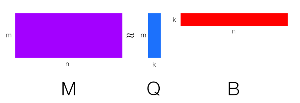
Since the above algorithm finds $Q$, we can in turn approximate $M$ with a low rank factorization of $M \approx Q B$ where $B = Q^T M$. That in and of itself can be very useful to shrink down datasets represented by $M$, given $k \ll m \leq n$.

Another use for this is when we want to perform Principle Component Analysis (PCA) on some matrix $M$. It turns out that the columns of $Q$ are actually the set of the $k$ dominant features vectors we can use to drop a dataset represented by $M$ to $k$ dimensions and $B$ is the dataset in the lower dimensional form. In practice, one would then use $B$ as the independent variable data that a model would be build from.

The badass thing about using the above algorithm for PCA is you get the same orthogonal features you would performing PCA via an SVD decomposition, but you avoid the computational cost of an SVD decomposition!

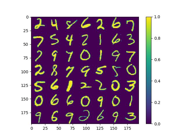
Just as an example, a dataset of $10,000$ images of handwritten digits from the MNIST dataset were used to test out dimensionality reduction using the above algorithm. Note that each image is made up of $784$ pixels, meaning each point in the dataset is $784$ dimensions. Now to give one an idea of how the dataset looks, the first figure below shows what a random set of digits might look like.

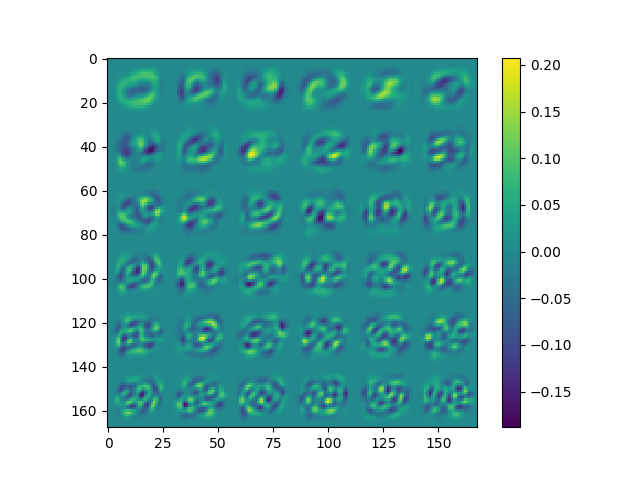
The second figure shows the $36$ features extracted using the randomized range finder algorithm, effectively making the dataset reducible to having $36$ dimensional data points instead of the original $784$ dimensional points!

The above example using this Randomized Range Finder is pretty cool and it certainly can be used in plenty more applications! For example, I personally have used the above algorithm as a stepping stone to building an efficient randomized SVD code.

Additionally, one can modify the above algorithm to be adaptive, meaning we do not need to specify some rank $k$, and can instead allow the algorithm to find the optimal value for $k$ given some tolerance. This can be very useful in the above examples so we can trade off accuracy with run-time/data compression.

Conclusion

As we saw in this post, there are methods we can use to estimate the range of some matrix. Using some pretty simple randomized approaches, we can make this estimation much more efficient at the expense of some minor approximation error. As shown, the resulting Randomized Range Finder can find use in many things, ranging from data compression to feature extraction and more. Basically, this algorithm is pretty cool!